Abstract
AI progress can feed back into AI research in two ways. Capability improvements allow AIs to perform a larger share of AI research tasks, while efficiency improvements raise AI research output per unit of compute on tasks already automated. In a task-based automation model, I show that a software intelligence explosion—a self-sustaining acceleration in AI progress with fixed compute and human labor—requires both margins to improve sufficiently fast, and neither margin can substitute for the other. To see whether these conditions hold, I calibrate both margins with data on recent AI progress. In my baseline estimation, both the capability and efficiency conditions for an SIE are met; however, efficiency progress is borderline, and uncertainty intervals include both conditions failing. In a Monte Carlo simulation over the parameter distribution, an SIE occurs in 49% of draws. These results indicate that an SIE is plausible but uncertain based on current trends in AI progress.
1 Introduction
Frontier AI systems are increasingly being used to accelerate R&D into future AI systems. This creates a positive feedback loop where the development of increasingly capable AI systems can aid in the development of even more advanced successor systems. Some version of this recursive self-improvement loop already operates today, with AI companies reporting internal research speedups from using AI (Favaro and Clark 2026; OpenAI 2026). If this loop becomes strong enough to sustain itself—accelerating AI progress even with no growth in compute or human researchers—the result would be a software-only intelligence explosion (SIE), potentially leading to runaway AI progress. Understanding the conditions for an SIE is one of the most important questions in AI today.
To establish the conditions for an SIE, I formalize a model of AI research in which AI progress feeds back into itself through two margins. Capability is the share of AI research tasks that AI can perform, while efficiency is AI research output per unit of compute on automated tasks. I use this model to establish the conditions for an SIE, and then calibrate the model with data on AI progress to see whether these conditions hold in recent AI progress.
The benchmark model of idea production (Jones 1995) summarizes research with a scalar stock of efficiency units. The pace of technological progress is entirely a function of this stock, with no distinction between types of researchers. In this representation, sufficiently many low-productivity researchers substitute for any high-productivity researcher. The same logic makes sufficiently many copies of a less capable AI a substitute for a more capable model (or human). For example, Alec Radford is a renowned AI researcher who led the development of OpenAI’s original GPT models. But the benchmark model implies there is some \(N\) such that \(N\) freshman computer-science majors do better AI research than Alec Radford. This is an implausible assumption in the context of AI research.
I replace scalar research progress with the task-based model of Aghion et al. (2019), applied to AI research itself, with compute in place of capital. AI progress feeds back into AI research through two channels. Capability improvements expand the set of AI research tasks that AI can successfully perform; efficiency improvements increase the amount of AI research labor supplied by a given compute stock, so they are analogous to population growth for automated researchers. The compute that matters for research automation is inference compute, the compute used to run trained AI models, as distinct from the training compute used to create them. I show that the speed of AI progress is determined by the slower of these two margins, so an SIE requires both margins to be sufficiently fast. Efficiency improvements alone eventually run into Baumol effects, where non-automated tasks bottleneck AI progress. Capability improvements alone fail because automating a larger share of tasks only spreads the fixed compute stock thinly across all tasks, without expanding the population of automated researchers.
In the second half of the paper, I quantify efficiency progress and capability progress using recent data on AI progress, to test whether the conditions for an SIE hold. Each leg of the SIE condition can be expressed as a ratio of an observable growth rate to the growth rate of research inputs, in the manner of the returns-to-software parameter of Eth and Davidson (2025). The efficiency leg is the rate of algorithmic efficiency progress on a fixed set of tasks, which I take from the literature. My main empirical contribution is to quantify capability growth in a way that connects to the conditions for an SIE. To do so, I use the time horizon measured by METR, an AI evaluation nonprofit: the length of task, in the time it takes a skilled human, that an AI model completes with 50% probability. On a suite of software and research tasks with measured human completion times, the time horizon of frontier models has doubled every four to seven months (METR 2026). Combining this horizon trend with the distribution of human completion times across tasks, and the assumption that this distribution has a Pareto tail, gives the growth rate of capabilities.
In my baseline calibration, point estimates imply both the efficiency and capability conditions for an SIE are met: capability returns are \(3.45\) (95% interval \(0.60\)–\(8.22\)), and efficiency returns are \(1.07\) (\(0.45\)–\(2.52\)). Thus, efficiency rather than capability is the binding constraint on an SIE, but the 95% intervals include both conditions failing. In a Monte Carlo simulation over the uncertainty in each input, I find that an SIE occurs in 49% of draws. Thus, an SIE is plausible.
This analysis is much more speculative than typical empirical research in economics, and it relies on many simplifying assumptions, both in the model and in mapping it to data. Section 6 discusses the main limitations.
The rest of the paper is organized as follows. Section 2 relates the paper to the literature. Section 3 lays out the model. Section 4 derives the two-legged condition for an SIE. Section 5 maps the model to data and estimates the two margins of progress. Section 6 concludes and discusses policy implications.
2 Related Literature
This paper is part of the still-too-small literature that models AI progress using endogenous growth theory. Canonically, these papers (Eth and Davidson 2025; Davidson and Houlden 2025; AI Futures Project 2025) have used a benchmark endogenous growth model in the style of Jones (1995), which measures research in scalar efficiency units and so elides the capability-efficiency distinction that I focus on. Some recent papers in this literature have taken a different path: Davidson et al. (2026) focus on networked spillovers and feedback loops in the macroeconomic setting, with AI as one sector in an economywide feedback loop, but they too measure research in scalar units.
There are two exceptions. First, Cunningham and Shetty (2026) model AI research as an apple-picking process, where AI can pick apples up to a certain “height”, corresponding to task automation in my model. However, they model AI labor as abundant, ignoring the efficiency dimension that I focus on. Second, Cunningham et al. (2026) apply a similar framework to model AI research automation; they do highlight the capability-efficiency distinction. However, they abandon the endogenous growth framework and rely only on reduced-form elasticities, whereas I derive elasticities from a task-based model. This requires more assumptions, but is better able to use historical data.
Methodologically, I use a task-based automation model, with similarities to others deployed in the literature, including those used to study the effect of AI on economic growth (Aghion et al. 2019; Jones and Tonetti 2026). The mechanics of my model are almost identical; the feedback loop over effective compute echoes the positive feedback from capital in a standard growth model, and many capital-accumulation mechanisms carry over to the setting of AI research. My main theoretical contribution is to show that the task automation structure implies a two-legged condition for an SIE. Secondarily, while previous papers start from the premise of full automation of AI research to derive the conditions for an SIE (Eth and Davidson 2025; Davidson and Houlden 2025), I derive conditions based on the speed of AI research automation, which is observable today.
Empirically, I draw on the literature that estimates AI progress: fixed-task estimates of algorithmic efficiency (Ho et al. 2024; Erdil and Besiroglu 2022; Gundlach, Fogelson, et al. 2025), the time-horizon measurements of Kwa et al. (2025) and METR (2026) and their decomposition into compute and software (Whitfill et al. 2025), and estimates of the substitutability of compute for research labor (Whitfill and Wu 2025). In calibrating the efficiency leg of AI progress, I largely rely on this literature. My main empirical contribution is to connect the growth of AI capabilities to data on the time horizons of tasks that AI can complete, and using this calibration to assess the likelihood of an SIE.
3 Model
AI development requires a continuum of research tasks \(i \in [0,1]\), to be performed by a fixed stock \(L>0\) of human researchers or a fixed stock \(Z>0\) of physical compute (on which copies of the frontier AI model run).2
A key feature of my model is that “compute” denotes inference compute used to run automated researchers. This is an important deviation from standard ways of thinking about the role of compute in AI progress. Compute is most commonly identified with training compute, because scaling laws suggest that scaling training compute increases AI capabilities. It is also sometimes identified with experimental compute, which could be a strong complement to research labor, and thus could bottleneck AI progress (Whitfill and Wu 2025). While both of these are reasonable uses of the term “compute”, neither is applicable to this model. This is an important restriction: it means that my model does not describe the conditions under which training compute bottlenecks or experimental compute bottlenecks could prevent an SIE. My model focuses only on the conditions for when AI cognitive labor can substitute for human cognitive labor. A full accounting of all the roles that compute plays in AI research, and an endogenous allocation between all of these roles, is left to future research.
3.0.0.1 AI progress.
The rate of change \(\dot{A}_t\) of frontier AI technology is driven by the level of current technology \(A_t\) and research output \(R_t\), as in the benchmark semi-endogenous model.
\[\begin{equation} \dot{A}_t \;=\; \delta\, R_t^{\lambda}\, A_t^{1-\beta}, \qquad \delta > 0,\ \beta > 0,\ 0 < \lambda \le 1 \tag{1}\end{equation}\]
Research output enters (1) with elasticity \(\lambda\), the stepping-on-toes parameter: when \(\lambda<1\), parallel research effort duplicates itself, so doubling \(R_t\) less than doubles the rate of progress. Technology enters with elasticity \(1-\beta\): doubling \(A_t\) less than doubles the rate of progress, representing ideas getting harder to find.
3.0.0.2 Research production.
AI research requires performing tasks indexed by \(i \in [0, 1]\). Research task \(i\) can either be human-only, or automatable (can be performed by AI). Task-specific output is given by
\[\begin{equation} r_t(i) \;=\; \begin{cases} \ell_t(i) + \nu(A_t)\, z_t(i), & i \le \alpha(A_t), \\[2pt] \ell_t(i), & i > \alpha(A_t) \end{cases} \tag{2}\end{equation}\]
Here, \(\nu(A_t)\) is efficiency, the task output that can be produced with one unit of compute on an automated task, and \(\alpha(A_t)\) is capability, the share of tasks that can be performed by AI at all; both depend on the level of AI technology, as specified below.
Tasks are complements in aggregate research output, being combined with a constant elasticity of substitution \(0<\sigma<1\): \[\begin{equation} R_t \;=\; \left( \int_0^1 r_t(i)^{\frac{\sigma-1}{\sigma}} \,\mathrm{d}i \right)^{\frac{\sigma}{\sigma-1}} \tag{3}\end{equation}\]
3.0.0.3 Capability and efficiency improvements.
Efficiency \(\nu\) and capability \(\alpha\) are determined by the level of AI technology:
\[\begin{equation} \alpha(A_t) = 1 - A_t^{-\mu}, \qquad \mu \ge 0,\ A_t \ge A_0 \ge 1, \tag{4}\end{equation}\]
\[\begin{equation} \nu(A_t) = c\, A_t^{\eta}, \qquad c > 0,\ \eta \ge 0 \tag{5}\end{equation}\]
Both of these equations parameterize capability and efficiency in terms of elasticities. \(\mu\) is the capability elasticity and \(\eta\) is the efficiency elasticity: a 1% increase in the technology level raises AI research input per unit of compute by \(\eta\)% and shrinks the human-only task share \(1-\alpha\) by \(\mu\)%.
Of course, parameterizing capability and efficiency this way assumes that their elasticities are constant, no matter the level of technology. This is a particularly important assumption when it comes to capability: Equation (4) implies that \(\alpha < 1\), and thus AI research is never fully automated. Eth and Davidson (2025) start from the premise of fully-automated AI research, and then derive the conditions for an SIE, so this may at first seem to preclude the possibility of an SIE. As I show below, this is not true; rather, it casts the condition for an SIE in terms of how fast capabilities grow instead of whether research has been fully automated, and the former is much easier to measure, which makes empirical analysis of an SIE more tractable.
Define effective compute as the AI research input supplied by physical compute at the current level of efficiency, \[X_t \;\equiv\; \nu(A_t)\, Z ,\] with units chosen so that \(X_t\) is measured in researcher-equivalents. Its physical component \(Z\) is a fixed stock, and its software component \(\nu(A_t)\) is produced by the loop itself.
Finally, the resource constraint is that researchers and physical compute applied across tasks exhaust the total available researchers and compute.
\[\begin{equation} \int_0^1 \ell_t(i) \,\mathrm{d}i \;=\; L, \tag{6}\end{equation}\] \[\begin{equation} \int_0^{1} z_t(i) \,\mathrm{d}i \;=\; Z \tag{7}\end{equation}\] Table 1 collects the environment.
| Block | Statement |
|---|---|
| Technology: law of motion | \(\dot{A}_t = \delta R_t^{\lambda} A_t^{1-\beta}\) |
| Technology: capability | \(1 - \alpha(A_t) = A_t^{-\mu}\) |
| Technology: efficiency | \(\nu(A_t) = c A_t^{\eta}\) |
| Research tasks | \(r_t(i) = \ell_t(i) + \mathbf{1}\{i \le \alpha(A_t)\} \cdot \nu(A_t)z_t(i)\) |
| Research aggregation | \(R_t = \big(\int_0^1 r_t(i)^{\frac{\sigma-1}{\sigma}} \,\mathrm{d}i\big)^{\frac{\sigma}{\sigma-1}}\) |
| Resources: researchers | \(\int_0^1 \ell_t(i)\,\mathrm{d}i = L\) |
| Resources: physical compute | \(\int_0^{1} z_t(i)\,\mathrm{d}i = Z\) |
To close the model, we need an allocation rule for labor and compute. I assume that the allocation is chosen to maximize aggregate research output \(R\), consistent with labor and compute being allocated internally to a profit-maximizing AI developer. Define research capacity as this maximized \(R^*\).
Proposition 1 (Task Allocation). Define \(\alpha^{*}\equiv \frac{X}{L+X}\). Research capacity is \[\begin{equation} R^*(\alpha; L, X) \;=\; \begin{cases} \left[\, \alpha^{\frac{1}{\sigma}} X^{\frac{\sigma-1}{\sigma}} + (1-\alpha)^{\frac{1}{\sigma}} L^{\frac{\sigma-1}{\sigma}} \,\right]^{\frac{\sigma}{\sigma-1}}, & \alpha \le \alpha^{*},\\[4pt] L + X, & \alpha \ge \alpha^{*}. \end{cases} \tag{8}\end{equation}\]
Below the threshold, research capacity is a CES aggregate of the two factor stocks: labor \(L\) and effective compute \(X\) enter (8) with the same elasticity of substitution \(\sigma\) as the tasks themselves, and with weights \(\alpha^{1/\sigma}\) on compute and \((1-\alpha)^{1/\sigma}\) on labor. Capability improvements act inside this aggregator: raising \(\alpha\) moves weight from labor to compute without changing either stock. Written in factor-augmenting form, the aggregate is a CES in \(\alpha^{-1/(1-\sigma)}X\) and \((1-\alpha)^{-1/(1-\sigma)}L\), the form in Aghion et al. (2019), so a capability improvement is equivalent to labor-augmenting technical change of size \((1-\alpha)^{-1/(1-\sigma)}\) on the fixed stock of researchers together with a dilution of compute over a larger task set. The labor-augmented term \(L(1-\alpha)^{-1/(1-\sigma)}\) is the most research the economy can produce at capability \(\alpha\) however abundant effective compute becomes (Lemma 1 in Appendix A.2), and it governs the capability leg of the explosion condition below.
The threshold \(\alpha^{*}= X/(L+X)\) is the point of full factor utilization. Past it, compute has been spread so thin that per-task AI input falls below what concentrated researchers supply elsewhere; researchers re-enter automated tasks until inputs equalize, and research capacity is just the total factor supply, \(L+X\).
4 Explosion Conditions
Definition 1 (Software Intelligence Explosion). Holding \(L\) and \(Z\) fixed, the model exhibits a software intelligence explosion if AI progress eventually raises the growth rate of the technology level, \(g_A = \dot A_t/A_t\), at a sustained proportional rate: \[\begin{equation} \liminf_{A\to\infty}\frac{\,\mathrm{d}\ln g_A}{\,\mathrm{d}\ln A}>0 \tag{9}\end{equation}\] Locally, acceleration occurs when \[\frac{\,\mathrm{d}\ln g_A}{\,\mathrm{d}\ln A}>0 \quad\Longleftrightarrow\quad \frac{\,\mathrm{d}\ln\dot A}{\,\mathrm{d}\ln A}>1\] The limit condition in (9) distinguishes a self-sustaining acceleration from a temporary rise in \(g_A\) or convergence to a constant growth rate.
Another reasonable definition of an SIE would be as a technological singularity, where \(A_t\) becomes infinite in finite time. In this model, there is no distinction; the results below hold for both definitions.
Proposition 2 (Asymptotic Growth). Define the efficiency returns, the capability returns and the binding returns as \[r_E\equiv\frac{\lambda\eta}{\beta},\qquad r_C\equiv\frac{\lambda\mu}{(1-\sigma)\beta},\qquad r^{*}\equiv\min\{r_E,r_C\}.\] Holding \(L\) and \(Z\) fixed, \[\begin{equation} \lim_{A\to\infty}\frac{\,\mathrm{d}\ln g_A}{\,\mathrm{d}\ln A}\;=\;\beta\,(r^{*}-1), \qquad\text{equivalently}\qquad \lim_{A\to\infty}\frac{\,\mathrm{d}\ln g_A}{\,\mathrm{d}\ln A^{\beta}}\;=\;r^{*}-1 . \tag{10}\end{equation}\]
The elasticity of research capacity with respect to technology converges to the smaller of two numbers: \(\eta\), the rate at which effective compute grows, and \(\mu/(1-\sigma)\), the rate at which the shrinking human-only task share relaxes its constraint on research. Duplication scales that elasticity by \(\lambda\), and idea difficulty subtracts \(\beta\). Integrating (1) gives \(A_t^{\beta}=A_0^{\beta}+\beta\delta\int_0^t R_\tau^{\lambda}\,\mathrm{d}\tau\), so \(A^{\beta}\) grows with cumulative research net of duplication, so the second form of (10) reads: each percent of cumulative research raises the growth rate by \(r^{*}-1\) percent. When \(r^{*}<1\) the growth rate falls at that rate and the technology level grows sub-exponentially.
The two ratios are the objects that matter for the empirical analysis in Section 5: the technology level has no natural units, so the elasticities \(\eta\), \(\mu\) and \(\beta\) are identified from data only up to a common scale and \(\lambda\) only jointly with them, whereas \(r_E\) and \(r_C\) are identified directly.
Corollary 1 (SIE Conditions). The model exhibits a software intelligence explosion if and only if \(r^{*}>1\), that is, \[\begin{equation} \boxed{\; \underbrace{\lambda\eta>\beta}_{\text{efficiency leg}} \quad\text{and}\quad \underbrace{\lambda\mu>(1-\sigma)\beta}_{\text{capability leg}} \; } \tag{11}\end{equation}\] The same conditions are necessary and sufficient for \(A_t\) to diverge in finite time. If \(r^{*}=1\), the growth rate converges to a positive constant.
Each inequality rules out a different failure. When either inequality fails strictly and is the tighter constraint, that margin eventually pulls the growth rate down.
Efficiency alone. Suppose efficiency improves fast enough to overcome idea difficulty, but capability does not: \(\lambda\eta>\beta\) but \(\lambda\mu\le(1-\sigma)\beta\). Productivity rises rapidly on automated tasks, but the complementary human-only task share contracts too slowly. Those tasks become an increasingly important share of the effective cost of research and eventually govern aggregate progress. This is the familiar Baumol effect, and the reason why Aghion et al. (2019) emphasize full automation as the condition for explosive economic growth: rapid progress in some tasks cannot sustain aggregate growth when essential laggard tasks remain.
Formally, research capacity never exceeds \(L(1-\alpha)^{-1/(1-\sigma)}\) (Lemma 1 in Appendix A.2), so for any efficiency path, \[\begin{equation} g_A \le \delta L^{\lambda} A^{\lambda\mu/(1-\sigma)-\beta} \tag{12}\end{equation}\] Since \(\lambda\mu/(1-\sigma)-\beta \le 0\) in this scenario, \(g_A\) is bounded by \(\delta L^{\lambda}\) at equality and falls to zero when the inequality is strict. Growth slows down as humans become the limiting factor.
Capability alone. The failure of capability improvements without efficiency improvements is more interesting, and is instructive about the difference between AI research and the economic growth context that this model is derived from. Capability improvements enter research capacity only through the weights in (8): they spread the fixed rival compute stock over a larger set of tasks, the dilution \(\alpha^{-1/(1-\sigma)}X\) in the factor-augmenting form above, but add no effective compute. The role of efficiency improvements is therefore analogous to the role of population growth in a semi-endogenous growth model: they are population growth for AI labor, expanding the number of automated researchers available to do AI research. Without them, the population of automated researchers is fixed, and a fixed population cannot generate exponential growth in a semi-endogenous model. This is why efficiency improvements are essential for sustained accelerations in AI progress.
Formally, research capacity never exceeds total factor supply, \(R^*\le L+X\) (Lemma 1), and effective compute is \(X=cZA^{\eta}\), so for any capability path \[\begin{equation} g_A \le \delta\,(L+cZA^{\eta})^{\lambda}\,A^{-\beta}, \tag{13}\end{equation}\] which falls to zero when \(\lambda\eta<\beta\) and is bounded by \(\delta(L+cZ)^{\lambda}\) when \(\lambda\eta=\beta\).
5 Calibration
5.1 Empirical Mapping
To map the theory to data, I first clarify the empirical counterparts to the model objects. In particular, “capability” and “efficiency” have subtle differences from the way these terms are ordinarily used. Eth and Davidson (2025) classify both acquiring new tasks and becoming more competent at tasks a system can already attempt as capability improvements, while achieving a given capability level with less compute is an efficiency improvement. Those definitions are intuitive, and useful for a broad accounting of software progress. But for the purpose of SIE accounting in this model, a different boundary is necessary.
5.1.0.1 Efficiency.
Efficiency is useful task output per unit of compute on automated tasks. The key feature of this definition is that the efficiency that matters for an SIE is inference efficiency, since that determines the quantity of AI labor available for AI research. Thus, the empirical counterpart I use is primarily the rate at which the inference compute needed to reach a fixed benchmark score has fallen (Gundlach, Lynch, et al. 2025), triangulated with estimates of efficiency progress based on pretraining (Section 5.3) even though these are not the relevant margin of efficiency progress.
The second important and unintuitive element of this definition is that improved quality at performing the same task is an efficiency improvement, rather than a capability improvement. If a model’s code quality improves for the same compute cost, this may seem like a capability improvement, but for SIE accounting it raises efficiency. Within a task, I assume that quality and cost are interchangeable, so that an AI that can do a task outstandingly well is isomorphic to an AI that can do that task adequately at low cost. Thus, the critique that motivated this model—that the standard model treats quality and quantity as interchangeable—still applies. However, it is a more palatable assumption at the task level than at the level of AI research as a whole. On the whole, this exercise largely tracks previous exercises that aim to calculate the returns to software progress as they relate to an SIE (see Table 4), and is not conceptually novel.
5.1.0.2 Capability.
In this model, capability is the automated task share \(\alpha\). Unlike efficiency, the automated share is not observed: there is no comprehensive enumeration of AI research tasks, let alone a record of which of them are automated. Favaro and Wright (2026) take a step in this direction: they catalogue Anthropic’s model R&D work into 378 task categories, weight each by the staff time spent on it, and rate how far each is automated. They publish only aggregate shares, however, not the task list or the per-task ratings, so their task set cannot be used here. So how can we measure the automated share of tasks?
Mapping the unobservable task share growth to observable quantities is my main empirical contribution. To do this, we have to augment the model of Section 3 with four assumptions.
Task length. Index each research task by a scalar difficulty \(q>0\), measured as the time a human expert needs to complete it (“task length”). Task length is distributed \(q\sim F\).
Capability threshold. A model at technology level \(A\) has some threshold difficulty \(h(A)\) such that it can perform every task with \(q\le h(A)\) and no task with \(q>h(A)\). Define \(h(A)\) as the model’s time horizon.3
Task measure. The continuum in (3) weights tasks by their labor requirement: a task that takes \(T\) hours occupies \(T\) units of researcher input. \(F\) is therefore the distribution of task length across work-hours, \(F(T)\) being the fraction of all task-hours in tasks with \(q\le T\), and the automated share is \(\alpha(A)=F(h(A))\).
Pareto tail. Above some length \(h_0\), \(F\) has a Pareto tail with index \(k>0\): \(1-F(T)=\bar F_0\,(T/h_0)^{-k}\) for \(T\ge h_0\), where \(\bar F_0\equiv1-F(h_0)\in(0,1]\).
Proposition 3 (Capability from Time Horizons). Under (a)–(d), for every technology level with \(h(A)\ge h_0\), \[\begin{equation} 1-\alpha(A)=\bar F_0\left(\frac{h(A)}{h_0}\right)^{-k}, \qquad \mu\;=\;k\,\frac{\,\mathrm{d}\ln h}{\,\mathrm{d}\ln A}, \tag{14}\end{equation}\] and along any path of AI progress the human-only task share shrinks at rate \[\begin{equation} g_\alpha\;\equiv\;-\frac{\,\mathrm{d}\ln(1-\alpha)}{\,\mathrm{d}t}\;=\;k\,g_h, \qquad g_h\equiv\frac{\dot h}{h}. \tag{15}\end{equation}\]
The intuition is that when we learn how the time horizon of AI models evolves, we learn which task lengths it can do with some threshold probability. If we further know how research work is spread across task lengths, we can convert a longer horizon into a larger automated share. The Pareto tail makes this conversion simple, because a Pareto distribution looks the same at every scale: each doubling of the horizon automates the same fraction of the work that still lies beyond it, whatever the current horizon. With \(k=1.31\), every doubling of the horizon automates about \(1 - 2^{-k} =\) 60% of the remaining human-only work. The human-only share therefore shrinks at a constant proportional rate, \(k\) times the growth rate of the horizon. Proposition 3 thus replaces the unobservable quantity \(\alpha(A)\) with two quantities \(k\) and \(g_h\) that can be estimated from the data. This solves our problem of estimating the growth rate of capabilities.
One final adjustment is needed before we can use the horizon trend to estimate capability progress. The observed time horizon growth reflects both software progress and the growth of training compute, but when studying an SIE we want to know the capability growth that came purely from software progress. We can attribute some share \(s\) of time horizon growth to software progress, so that the software-attributable horizon growth \(s\,g_h\) is what enters the capability leg.
5.2 Identification
The parameters \(\eta\), \(\mu\), \(\beta\), \(\lambda\) are defined relative to the technology level \(A\), which has no natural units. Only the combinations \(\lambda\eta/\beta\) and \(\lambda\mu/\beta\) are identified from data, and Corollary 1 states the SIE conditions in exactly those combinations, \(r_E>1\) and \(r_C>1\). In the data we can observe three growth rates that map into the model:
the efficiency growth rate \(g_\nu\equiv\dot\nu/\nu=\eta g_A\)
the rate \(g_\alpha=\mu g_A\) at which the human-only task share shrinks
the growth rate of research capacity \(g_R\equiv\dot R/R\).
Then the SIE condition—expressed in terms of these growth rates and the observable parameters of the model—is:
Proposition 4 (Returns Ratios). Suppose that over a historical window research capacity and technology grow at constant rates \(g_R>0\) and \(g_A\). Then \(\beta g_A=\lambda g_R\), the returns of Proposition 2 are ratios of observable growth rates, and the SIE conditions of Corollary 1 read \[\begin{equation} \boxed{\; r_E\;=\;\frac{g_\nu}{g_R}\;>\;1 \quad\text{and}\quad r_C\;=\;\frac{g_\alpha}{(1-\sigma)\,g_R}\;>\;1 \;} \tag{16}\end{equation}\]
Both legs are returns parameters. The efficiency returns \(r_E\) count the doublings of efficiency per doubling of cumulative research input along a balanced path, which is the returns-to-software parameter \(r\) of Eth and Davidson (2025) and Davidson and Houlden (2025) applied to inference efficiency. The capability returns \(r_C\) are slightly more complicated. They count the doublings of the inverse human-only share \(1/(1-\alpha)\) per doubling of cumulative research input. Moreover, this is measured against the threshold \(1-\sigma\) rather than \(1\): the more complementary tasks are, the faster the human-only share must shrink to keep up.
Proposition 3 further gives \(g_\alpha=k\,g_h\); with compute held fixed the relevant horizon growth rate is \(s\,g_h\), so the capability leg reads \[\begin{equation} r_C=\frac{k\,s\,g_h}{(1-\sigma)\,g_R} . \tag{17}\end{equation}\]
The calibration uses six inputs, listed with their baselines and ranges in Table 2.
| Symbol | Input | Baseline | Range | Distribution |
|---|---|---|---|---|
| \(g_\nu\) | Fixed-task efficiency growth | 0.92 | 0.42–2.02 | log-normal |
| \(g_R\) | Research labor growth | 0.86 | 0.64–1.15 | log-uniform |
| \(g_h\) | Time-horizon growth (50%) | 1.93 | 1.57–2.36 | log-normal |
| \(s\) | Software share of horizon growth | 0.46 | 0.31–0.71 | uniform |
| \(k\) | Task-length tail index | 1.31 | 0.52–1.87 | log-uniform |
| \(\sigma\) | Task substitution elasticity | 0.61 | 0.00–0.83 | uniform |
5.3 Efficiency Leg
5.3.0.1 Efficiency progress \(g_\nu\).
Unlike the returns-to-software estimates of Eth and Davidson (2025) and Davidson and Houlden (2025), which use pretraining efficiency, the numerator of \(r_E=g_\nu/g_R\) is primarily inference efficiency. I pool four estimates of algorithmic efficiency progress at a fixed task and performance level (Appendix B.1 gives each source). The primary estimate measures the right object: the decline in the inference compute needed to reach a fixed score on GPQA Diamond, a benchmark of graduate-level science questions, net of hardware improvements, which Gundlach, Lynch, et al. (2025) infer from the prices of open-weight models. It is \(1.17\) per year. Because it is identified from a small set of open models over a short period, I triangulate it with three training-side estimates and pool the four; Appendix B.1 describes the sources, the weights and the pooling. The baseline is \(g_\nu=0.92\).
5.3.0.2 Research inputs \(g_R\).
Staff at frontier laboratories has grown rapidly since the release of ChatGPT in late 2022. Ho and Whitfill (2025) report a growth rate of 0.85 log points per year in OpenAI’s staff count, approximately \(2.3\times\) per year. Davidson et al. (2026) report growth in AI-laboratory headcount of roughly \(140\%\) per year since ChatGPT (i.e. \(\ln 2.4\approx0.88\) log points per year), from Epoch AI data. I set a baseline of \(g_R=0.86\) log points per year. Note also that since \(g_R\) is the denominator of both returns ratios, it appears in both SIE conditions.
5.4 Capability Leg
5.4.0.1 Tail index \(k\).
I estimate \(k\) from the human completion times of the 96 tasks on which METR measures time horizons, in its Time Horizon 1.1 release, whose lengths come from timed attempts by skilled human professionals (METR 2026). Because the horizon trend is measured on the same suite, both objects in \(g_\alpha=k\,g_h\) refer to one distribution. The baseline is \(k=1.31\), with a range from \(0.52\) to \(1.87\). Appendix B.2 describes the sample, the estimator, the alternative datasets and the fits, and Figure 2 plots the fitted tail.
5.4.0.2 Task time-horizon growth \(g_h\).
The 50% time horizon is the task length at which a model’s fitted success probability is one half (Kwa et al. 2025).4 On METR’s updated Time Horizon 1.1 suite, the frontier time horizon has doubled every 196 days over 2019–2025 (95% confidence interval 162 to 223 days), and every 131 days since 2023 (107 to 161 days) (METR 2026). I use the faster post-2023 doubling times as the basis for \(g_h=1.93\), because this better captures the window in which frontier AI systems have been applied to research tasks.
5.4.0.4 Substitution elasticity \(\sigma\).
The model’s \(\sigma\) is the substitutability between research tasks, and by Proposition 1 also between effective compute and research labor below the threshold \(\alpha^{*}\). Calibrated models of AI-driven growth set the task elasticity between \(0.5\) and \(0.67\) (Davidson 2023; Erdil et al. 2025; Korinek and Suh 2024), drawing on aggregate estimates of substitution between capital and labor, and estimates of the elasticity of substitution between research compute and research labor range from Leontief to substitutes (Whitfill and Wu 2025). I set a baseline of \(\sigma=0.61\), the value in GATE, Epoch AI’s integrated assessment model of AI automation (Erdil et al. 2025), with a range from \(0\), the Leontief limit, to \(0.83\), the upper bound of the GATE range (Appendix B.2).
5.5 Monte Carlo Simulation
To quantify uncertainty in this calibration, I use Monte Carlo simulations that account for the uncertainty in each input. I draw the six inputs from the distributions in Table 2. The efficiency rate \(g_\nu\) is drawn from the pooled log-normal (21) of Appendix B.1; its median is the baseline. The horizon rate \(g_h\) is log-normal with median at the baseline and dispersion set by its confidence interval; \(g_R\) and \(k\) are log-uniform on their ranges, with the range for \(g_R\) symmetric in logs around the baseline; \(s\) and \(\sigma\) are uniform on theirs. The inputs are drawn independently of one another, since they come from unrelated data sources, but the two ratios are not independent: each draw’s \(g_R\) is the denominator of both, so a draw with slow input growth raises \(r_E\) and \(r_C\) together. I take 200,000 draws and report, for each returns ratio, its median, its 95% interval (the 2.5th to the 97.5th percentile) and the share of draws in which it exceeds one, together with the share of draws in each combination of legs holding.
Finally, I do a variance decomposition to explore where the primary sources of uncertainty are. Because both log ratios are sums of independent terms, the variance of each decomposes exactly into input contributions, a fact I exploit to interpret the results.
5.6 Results
Table 3 collects the headline results. An SIE requires both returns to exceed one (Corollary 1).
| Monte Carlo | ||||
|---|---|---|---|---|
| Baseline | Median | 95% interval | Share above one | |
| Efficiency returns \(r_E\) | 1.07 | 1.07 | 0.45–2.52 | 56% |
| Capability returns \(r_C\) | 3.45 | 2.01 | 0.60–8.22 | 85% |
| Binding returns \(r^{*}=\min\{r_E,r_C\}\) | 1.07 | 0.99 | 0.44–2.21 | 49% |
| Share of Monte Carlo draws in which | ||||
| both legs hold (an SIE) | 49% | |||
| only the capability leg holds | 37% | |||
| only the efficiency leg holds | 7% | |||
| neither leg holds | 7% | |||
5.6.0.1 Efficiency leg.
At baseline, \(r_E=0.92/0.86=1.07\), with a 95% Monte Carlo interval of \(0.45\) to \(2.52\). Estimates that pool across performance levels or stitch benchmarks into a capability index report \(6\times\) to \(10\times\) per year (Ho et al. 2025; Ho 2026); in the numerator they would raise \(r_E\) to between \(2.1\) and \(2.7\). Table 4 places the ratio among published estimates of returns to software research, whose central estimates all lie between \(0.8\) and \(4\).
| Source | Central | Range | Basis |
|---|---|---|---|
| This paper | 1.07 | 0.45–2.52 | Section 5.3 |
| Eth and Davidson (2025) | — | 1–4 | domain doubling times over input growth |
| Davidson and Houlden (2025) | 1.2 | 0.4–3.6 | computer vision |
| Erdil et al. (2024) | 0.83 | 0.53–1.12 | computer chess |
| Ho and Whitfill (2025) | 1.89 | 1.07–3.21 | language models |
| Ho and Whitfill (2025) | 1.26 | 0.73–2.09 | computer vision |
Erdil et al. (2024) report only a bootstrap standard error of 0.15, from which this confidence interval is constructed via normal approximation.
5.6.0.2 Capability leg.
At baseline, \(r_C=k\,s\,g_h/((1-\sigma)\,g_R)=3.45\), with a 95% Monte Carlo interval of \(0.60\) to \(8.22\): the human-only task share shrinks \(3.45\) times as fast as the capability leg requires.
5.6.0.3 Joint uncertainty.
At baseline the efficiency leg sits just above the threshold and the capability leg is well clear of it. In the Monte Carlo simulations plotted in Figure 1, both legs hold in 49% of draws. The capability leg alone holds in 37%, so that efficiency binds; the efficiency leg alone holds in 7%, so that capability binds; neither holds in 7%.
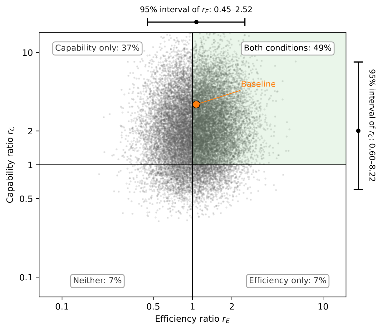
Notably, the 95% intervals of both returns ratios contain one: \(0.45\) to \(2.52\) for the efficiency returns and \(0.60\) to \(8.22\) for the capability returns. This variability highlights the inherent uncertainty of my setting; even capability progress, whose point estimate seems numerically all-but-guaranteed to be sufficient for an SIE, cannot be ruled sufficient with the standard of rigor usually applied to empirical research.
A feature of these results is that the median binding return is \(r^{*}=0.99\), with a 95% interval of \(0.44\) to \(2.21\). Thus, while both of the returns ratios are estimated to be above one, the binding ratio is on average less than 1. Thus, even though each condition holds on average, they do not hold together on average. Of course, given the amount of uncertainty in this data, there is no meaningful difference between \(0.99\) and \(1.07\). This is simply a demonstration of the importance of separating the efficiency and capability dimensions of an SIE, since focusing on only one of them would overstate the likelihood of an SIE.
5.6.0.4 Sources of uncertainty.
Table 5 decomposes the variance in the simulations into each input. The capability leg’s uncertainty is dominated by the substitution elasticity between research tasks, which supplies 49% of the variance of \(\ln r_C\), and the tail index, which supplies 30%, while the other parameters are much less important. The efficiency leg’s uncertainty primarily comes from the rate of efficiency progress in the numerator, which provides 85% of the variance of \(\ln r_E\). Interestingly, the standard deviation of \(\ln r_C\) is larger than that of \(\ln r_E\), yet the capability leg holds in more draws, because its median lies far above the threshold while the efficiency leg’s median lies just above it.
Because \(r_E\) is the most pivotal ratio for determining whether we are in an SIE regime or not, and its most uncertain input is the growth rate of efficiency \(g_\nu\), \(g_\nu\) is the parameter with the single largest contribution to uncertainty around the likelihood of an SIE. My results suggest that more investment into better measures of \(g_\nu\) would have high value-of-information, given the wide range implied by existing estimates.
| Input | share of \(\mathrm{Var}(\ln r_E)\) | share of \(\mathrm{Var}(\ln r_C)\) |
|---|---|---|
| \(g_\nu\) | 0.85 | — |
| \(g_R\) | 0.15 | 0.06 |
| \(g_h\) | — | 0.02 |
| \(s\) | — | 0.12 |
| \(k\) | — | 0.30 |
| \(\sigma\) | — | 0.49 |
| Standard deviation of \(\ln r\) | 0.44 | 0.68 |
6 Conclusion
I separate two margins of AI progress that the benchmark model of idea production merges: capability, the share of AI research tasks that AI can perform, and efficiency, the AI research output that a unit of compute supplies on those tasks. A software intelligence explosion requires both margins to improve fast enough relative to idea difficulty, and each leg of that condition is a returns ratio measurable from observable growth rates, over a historical window in which compute and AI inputs also grew.
A striking feature of these results is that the likelihood of being in an SIE, 49% of draws, is less than the likelihood of either condition holding on its own (56% for efficiency and 85% for capability). This highlights the two-legged nature of the condition: an SIE requires both margins to improve fast enough at once, so assessing either leg in isolation overstates how likely an SIE is. My analysis should therefore be taken as evidence for the plausibility of an SIE, while highlighting its fragile nature and reliance on multiple margins of progress.
These results also identify where policy could act. For a policymaker who wants to pace the frontier and slow AI progress, efficiency is the bottleneck target. The efficiency leg is necessary for an SIE, no matter how fast capability improves, and it is the leg that is closest to binding at baseline. A cap on efficiency progress that holds the efficiency returns at or below one, so that each doubling of cumulative research input yields at most one doubling of efficiency, rules out an SIE in the model, however fast capability improves. How much efficiency growth such a cap removes depends on how fast efficiency is in fact growing. At the baseline estimate, it requires lowering the efficiency returns by about 6%. The same logic applies to a policymaker who simply wants to control the pace of AI progress rather than prevent an SIE. The asymptotic acceleration of AI progress is governed by the binding returns \(r^{*}=\min\{r_E,r_C\}\) (Proposition 2), so any reduction in the efficiency returns lowers \(r^{*}\) directly, whereas a reduction in the capability returns changes it only once they fall below the efficiency returns. Thus, regulation to slow frontier AI progress could prioritize efficiency slowdowns over capability slowdowns.
This analysis is considerably more speculative than is standard in economics research, so I want to qualify these conclusions with the inherent limitations of my approach. First, this model takes a simplified view of compute. Compute enters the AI research process only as inference compute that serves AI research labor, with no distinction between the types of compute an intelligence explosion would draw on. Critically, experimental compute, one of the biggest potential bottlenecks to an SIE, appears nowhere in the model. This paper is best understood as a theory of how AI labor can contribute to an SIE, not a complete accounting of the role that compute would play in an SIE.
Second, the data used in this empirical exercise is both individually weak and also somewhat cobbled together. For example, the data on efficiency progress are noisy, with estimates of the rate of progress varying by an order of magnitude across sources. Furthermore, the relevant growth rates are computed over different periods—for example, the growth rate of research labor is measured largely since late 2022, while the inference efficiency growth rate is measured over April 2024 to November 2025, making a mismatched ratio. These are all empirical limitations inherent to the fast-moving setting of AI research, and they could influence the conclusions of my analysis.
Finally, this paper is not about the full automation of research. The model keeps a positive human-only task share at every technology level, so it is unsuited to analyzing what would happen if AI research were fully automated. Some experts expect AI research to be close to fully automated within the next few years (AI Futures Project 2025), and a different model would be needed to analyze the effects of AI progress in such a setting.
References
GovAI, karthik.tadepalli@governance.ai. This paper benefited greatly from the feedback of Sam Manning, Cheryl Wu, Alan Chan, Markus Anderljung, Tom Davidson, Phil Trammell, Tom Cunningham, Joseph Levine, Kris Gulati, and audiences at OpenAI, GovAI and Forethought. Remaining errors are my own.↩︎
I hold physical compute fixed because on the short timescales for which people worry about an SIE, compute is unlikely to be part of the feedback loop.↩︎
Ord (2025)’s model of success rates over a time horizon provides a microfoundation for this step: a constant hazard of failure per unit of human task-time makes a model’s success probability fall monotonically with task length, so a single length \(h(A)\) separates the tasks a model completes at a given reliability from those it does not. The tail object there is the within-task survival curve; here it is the cross-task distribution \(F\).↩︎
The cutoff success probability changes the level of the horizon but not its growth rate: Kwa et al. (2025) report identical doubling times for 50% and 80% time horizons. Since only the growth rate enters the capability ratio, it doesn’t matter what cutoff we use.↩︎